Linear regression in vanilla Python with NumPy

This post covers how to do (multivariate) linear regression with Python using NumPy.

There are probably a dozen libraries which can do this for you but I just wanted to write this down since it's very easy to do it yourself. It's can also serve as a gentle introduction to NumPy (and to linear regression). Also, linear regression should probably be the first machine learning model you try when you get your hands on some data.

You can check out an example of using linear regression with some real world data in my previous post about estimating performance in power plants.

A quick review of linear regression

Linear regression is a statistical model to relate one or more explanatory variables $x_1, \ldots, x_p$ to a single (scalar) response variable $y$. The assumption of the model is that the response variable is a linear combination of the explanatory variables:

$$y = \beta_1 x_1 + \beta_2 x_2 + \ldots + \beta_p x_p.$$

The above is normally written in matrix notation as $y = \mathbf x^\top \boldsymbol \beta$, where $\top$ is the transpose, $\mathbf x = (x_1, \ldots, x_p)$ and $\boldsymbol \beta = (\beta_1, \ldots, \beta_p)$. Any disagreement between that and the reality is modeled through an error variable $\varepsilon$ so that the full model takes the form:

$$y = \mathbf x^\top \boldsymbol \beta + \varepsilon.$$

If we have $n$ observations of the data we can arrange the dependent variables in an $n \times p$ matrix and write

$$\mathbf y = \mathbf X \boldsymbol \beta + \boldsymbol \varepsilon.$$

That, up to here, is the linear regression model. From here on, there are several ways to estimate the values for the model parameters $\boldsymbol \beta$. All of them require you to make certain assumptions on the data and/or the errors. We'll look at the most popular and easiest one: the ordinary least squares estimate.

To estimate the parameters using this method we make the following assumptions:¹ - The design matrix $\mathbf X$ has full column rank. - All the errors are independent and identically distributed according to a zero-mean normal distribution with variance $\sigma^2$, i.e. $\varepsilon_i \sim N(0, \sigma^2)$. We'll assume the value for $\sigma^2$ is known (or you can estimate it from the data).

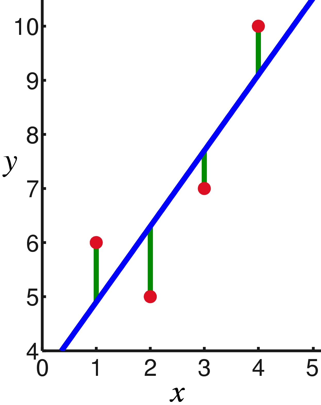
The ordinary least squares method finds estimates for $\boldsymbol \beta$ by minimizing

$$S(\boldsymbol \beta) = \lVert \mathbf y - \mathbf X \boldsymbol \beta \rVert^2.$$

Under the above assumptions, the optimal estimate is

$$\hat{\boldsymbol \beta} = (\mathbf X^\top \mathbf X)^{-1} \mathbf X^\top \mathbf y.$$

Python implementation

Without further ado, we're ready to look at how to implement this in Python using NumPy to do the matrix multiplication. We'll also use pandas to load the data.

Suppose we have a CSV file with one row per observation where the first column is the response variable and the rest are the dependent variables. We load it into a NumPy 2D array with

import pandas
import numpy as np

data = pandas.read_csv('data.csv')
X = data.iloc[:, 1:].to_numpy()
y = data.iloc[:, 1].to_numpy()[:, np.newaxis]

That'll give us the design matrix X and the response variable y as a column vector.

The computing the least squares estimate is just a matter of implementing the above formula:

beta_hat = np.linalg.inv(X.T @ X) @ X.T @ y

That'll return the parameter estimates as a column vector.

Bonus: adding a bias parameter

It's common to want to add a bias parameter that makes the linear regression an affine function, i.e. modelling an observation by adding a $\beta_0$ coefficient so that

$$y = \beta_0 + \beta_1 x_1 + \ldots \beta_p x_p.$$

That doesn't actually require any changes on the model, just add a variable dependent variable $x_0$ and always set it to $1$ and re-index. That's what I'd do in NumPy as well:

X_new = np.append(np.ones((X.shape[0], 1)), X, axis=1)

This will return a matrix where the first column is made up of ones and therefore the first coordinate of your beta_hat estimate will be that bias factor.