How hard is it to make a computer find peaks in audio signals?
by Elias Hernandis • Published April 27, 2020 • Tagged signal-processing, python, maths
TL;DR: very hard, it appears.
Feel free to play along with the Jupyter notebook and audio sample used for this experiment:
Suppose you have an audio signal and you want to detect peaks in it. Maybe you want to identify the beat in a song or you are trying to parse Morse code. In these situations you have a series of impulses which you can tell are louder than the rest of the audio. Even just by looking at the waveform, it is easy to tell that there is a peak in volume. Is it easy for a computer to do the same?
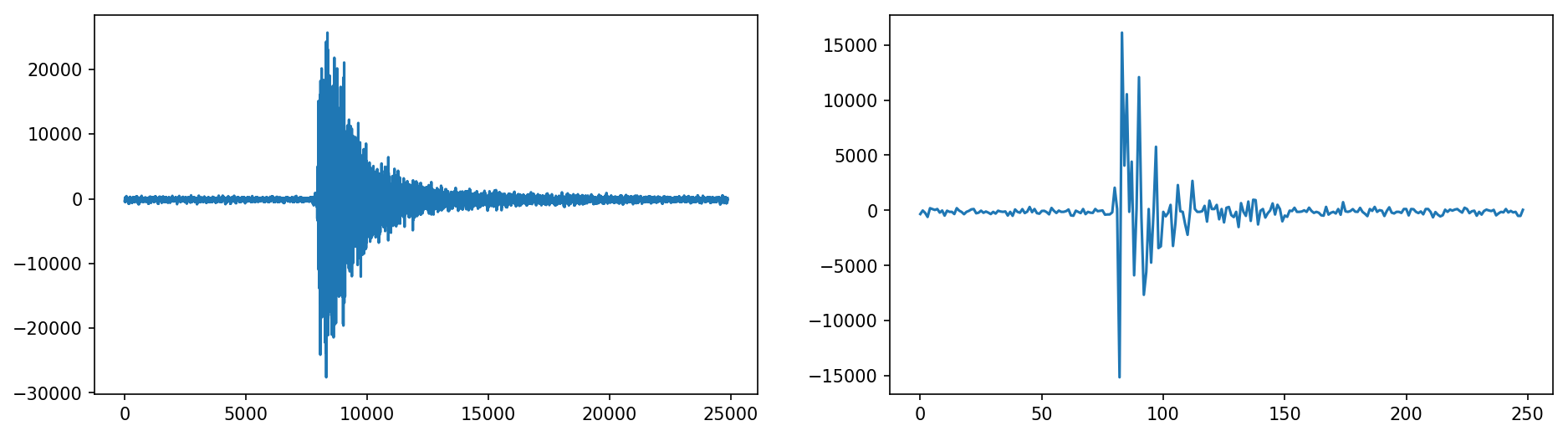
The pulses we are interested in1 look like the ones above. In this representation we are looking at time on the horizontal axis versus amplitude on the vertical axis. The raw signal is shown in the left graph, but there are so many data points that it almost looks like it has area under it. This is just an artifact produced by the lines that we use to visualize the waveform which join the data points. In the version to the right we have discarded 99% of the samples so that the fact that this is indeed a wave is clearer.
Back to our task of detecting peaks, our first idea is to find the local maxima of the wave function (recall that we are just looking at one peak of many, so we are indeed looking for several maxima). This is relatively easy to do: a sample is a local maximum if and only if it is bigger than the two samples adjacent to itself. Also, before proceeding any further, the function is almost symmetric with respect to the horizontal axis, so we can discard the negative part which will make things easier later 2:
def peaks1(x):
    res = []
    for i, v in enumerate(x[1:-1]):
        if x[i] < v and v > x[i + 2]:
            res.append((i, v))
    return res

# discard negative part
data1 = np.abs(mono)

print(f'{len(peaks1(mono))} out of {nsamples} are peaks')

#> 5921 out of 24863 samples are peaks
This first attempt reveals that around 25% of the samples are considered peaks under this definition of maximum. While this is not very useful in itself, we have uncovered that the signal is indeed very, very wiggly. We can try to smooth it out by computing a moving average and working with that instead. In our context, the audio signal is a sequence of around 25000 values A moving average of window size assigns to each point the average of the last points:
We need to be careful with the first values, since there is not enough history to calculate the average. Similarly, there wont be enough future to calculate the average for the last values. This can be a bit tedious to implement, especially with these last edge cases. We can leverage the fact that convolving the signal with a boxcar function of width and height will yield the same results and that NumPy already implements discrete convolutions and properly hadles the aforementioned edge cases.
W = 1000
data2 = np.convolve(data1, np.ones(W), 'valid') / W

In the above plot and the ones that follow, we have also taken the chance and reduced the number of points we are using for the plots, since we have already realised that the data is super wiggly. The original data is still used for the analysis, though.
If we now try to find the peaks we get
4585 out of 24863 samples are peaks
That is only a 20% reduction and we have used a window of 1000 samples! Even if we increase the window size (double it, even triple it), we still get thousands of peaks. Increasing the window size is not something desirable, since we can miss peaks that are close together but still "true" peaks that we want to identify. Clearly, convolution is not helpful enough? But... what if we do it once more?
data3 = np.convolve(data2, np.ones(W), 'valid') / W

Alright, the peak is slowly shifting to the left, but we don't care about that so much now, as long as we can find a peak:
31 out of 24863 samples are peaks
Okay, this has improved dramatically, but we still get 31 peaks when we would want to get just one. There must be a better way to do this but for the sake of completeness let's convolve a third time:
3 out of 24863 samples are peaks
While we are getting somewhere, this is taking way too much effort for our simple test with just one peak. We are still not able to count just one big peak. However, we are throwing away a ton of information: how big are these peaks, how far apart are they... Let's look at the three biggest peaks reported after each convolution:
1st convolution:  [(8046, 5412.995), (8056, 5403.334), (8033, 5394.965)]
2nd convolution:  [(7640, 4603.345313), (17143, 245.45059499999996), (18329, 219.05746100000002)]
3rd convolution:  [(7174, 4303.5119952939995), (16566, 241.88337264500004), (2165, 189.47858628800003)]
In the above output, each peak is represented by a tuple (time offset, peak height). There is something very interesting going on:
- As we expected, there is a shift to the left in the highest reported peak. This is an artifact of the convolution and will not be a problem if we just want to count how many peaks there are.
- The first convolution barely yields any results. For one, the first three peaks are equally high and very close together. Of course this tells us that there is a peak around there, but not how it relates to the rest of the signal without looking at the whole of the peak list.
- The second convolution clearly calls a dominant peak. The other two who made it to the top three are both far apart and much lower.
- Although the last (third) convolution reduces the number of peaks, it probably is not worth it since after we detect a dramatic increase in peak height from the first to the second detected peak after the second convolution we already have a candidate for mount Everest.
One possible reason for the dramatic increase in peak discrimination between the first and the second convolution is that data is much less wiggly (even though it still oscillates quite a lot) after the first convolution. This leads us to the question: do we need such a big window size for the second convolution? The answer appears to be no. Choosing a window size of 50 samples (as opposed to the 1000 we took for the first convolution) yields very similar results but with much less left-shift in the time coordinate where the peak is called:
1st convolution:  [(8046, 5412.995), (8056, 5403.334), (8033, 5394.965)]
2nd convolution, smaller window:  [(8014, 5386.55954), (10938, 926.6066200000001), (10927, 926.48548)]
Concluding remarks
This first look at the problem tells us that we cannot use the definition of a maximum common in Maths to find peaks in a waveform right away (precisely because it's a wave and we are looking for bigger scale features). It also tells us that the problem can be greatly simplified by reducing the wiggly-ness of the data (via convolution or some other method) and that we may not need to go all the way until we find a single peak in a desired region if we introduce some notion of peak prominence. A more detailed characterization of this concept of prominence has the potential to reduce the number and scale of convolutions needed to be able to call peaks. Also, we have encountered an artifact of this method where the time at which a peak is called shifts to the left with the number of convolutions performed. This is due to the asymmetric nature of the peaks we are dealing with, which may also prove to be determinant in our quest for peaks in audio signals.
P.S. Today is Koningsdag here in The Netherlands but sadly we cannot celebrate because of corona. At least Mathematics is always there with you.
-
This is not just one random pulse. The other day I had an idea which involves counting pops in audio and fitting the time it takes for the things to pop into a normal distribution. I hate eating raw corn. ↩
-
A more rigorous approach would have calculated the RMS value for tiny slices to reflect sound pressure more accurately. ↩